How Elasticsearch calculates significant terms

Image may be NSFW.
Clik here to view.

The magic of the “uncommonly common”.

Many of you who use Elasticsearch may have used the significant terms aggregation and been intrigued by this example of fast and simple word analysis. The details and mechanism behind this aggregation tends to be kept rather vague however and couched in terms like “magic” and the commonly uncommon. This is unfortunate since developing informative analyses based on this aggregation requires some adaptation to the underlying documents especially in the face of less structured text. Significant terms seems especially susceptible to garbage in – garbage out effects and developing a robust analysis requires some understanding of the underlying data. In this blog post we will take a look at the default relevance score used by the significance terms aggregation, the mysteriously named JLH score, as it is implemented in Elasticsearch 1.5. This score is especially developed for this aggregation and experience shows that it tends to be the most effective one available in Elasticsearch at this point.

The JLH relevance scoring function is not given in the documentation. A quick dive into the code however and we find the following scoring function.

Image may be NSFW.
Clik here to view.

Here the Image may be NSFW.
Clik here to view. is the frequency of the term in the foreground (or query) document set, while Image may be NSFW.
Clik here to view. is the term frequency in the background document set which by default is the whole index.

Expanding the formula gives us the following which is quadratic in Image may be NSFW.
Clik here to view..

Image may be NSFW.
Clik here to view.

By keeping Image may be NSFW.
Clik here to view. fixed and keeping in mind that both it and Image may be NSFW.
Clik here to view. is positive we get the following function plot. Note that Image may be NSFW.
Clik here to view. is unnaturally large for illustration purposes.

Image may be NSFW.
Clik here to view.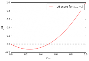

On the face of it this looks bad for a scoring function. It can be undesirable that it changes sign, but more troublesome is the fact that this function is not monotonically increasing.

The gradient of the function:

Image may be NSFW.
Clik here to view.

Setting the gradient to zero we see by looking at the second coordinate that the JLH does not have a minimum, but approaches it when Image may be NSFW.
Clik here to view. and Image may be NSFW.
Clik here to view. approaches zero where the function is undefined. While the second coordinate is always positive, the first coordinate shows us where the function is not increasing.

Image may be NSFW.
Clik here to view.

Furtunately the decreasing part of the function is in an area where Image may be NSFW.
Clik here to view. and the JLH score explicitly defined as zero. By symmetry of the square around the minimum of the first coordinate of the gradient around Image may be NSFW.
Clik here to view. we also see that the entire area where the score is below zero is in this region.

With this it seems sensible to just drop the linear term of the JLH score and just use the quadratic part. This will result in the same ranking with a slightly less steep increase in score as Image may be NSFW.
Clik here to view. increases.

Image may be NSFW.
Clik here to view.

Looking at the level sets for the JLH score there is a quadratic relationship between the Image may be NSFW.
Clik here to view. and Image may be NSFW.
Clik here to view.. Solving for a fixed level Image may be NSFW.
Clik here to view. we get:

Image may be NSFW.
Clik here to view.

Where the negative part is outside of function definition area.
This is far easier to see in the simplified formula.

Image may be NSFW.
Clik here to view.

An increase in Image may be NSFW.
Clik here to view. must be offset by approximately a square root increase in Image may be NSFW.
Clik here to view. to retain the same score.

Image may be NSFW.
Clik here to view.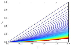

As we see the score increases sharply as Image may be NSFW.
Clik here to view. increases in a quadratic manner against Image may be NSFW.
Clik here to view.. As Image may be NSFW.
Clik here to view. becomes small compared to Image may be NSFW.
Clik here to view. the growth goes from linear in Image may be NSFW.
Clik here to view. to squared.

Finally a 3D plot of the score function.

Image may be NSFW.
Clik here to view.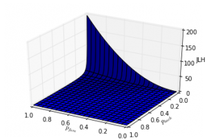

So what can we take away from all this? I think the main practical consideration is the squared relationship between Image may be NSFW.
Clik here to view. and Image may be NSFW.
Clik here to view. which means once there is significant difference between the two the Image may be NSFW.
Clik here to view. will dominate the score ranking. The Image may be NSFW.
Clik here to view. factor primarily makes the score sensitive when this factor is small and for reasonable similar Image may be NSFW.
Clik here to view. the Image may be NSFW.
Clik here to view. decides the ranking. There are some obvious consequences from this which would be interesting to explore in real data. First that you would like to have a large background document set if you want more fine grained sensitivity to background frequency. Second, foreground frequencies can dominate the score to such an extent that peculiarities of the implementation may show up in the significant terms ranking, which we will look at in more detail as we try to apply the significant terms aggregation to single documents.

The results and visualizations in this blog post is also available as an iPython notebook.